A fourth-order beam PINN in PyTorch
A beam-bending residual needs a fourth spatial derivative. This tutorial computes it through forward Taylor jets and trains the network with ordinary parameter autodiff. It solves a complete boundary-value problem with an independent analytic reference.
Solve a clamped Euler–Bernoulli beam with a nonuniform load, forward Taylor jets, exact boundary conditions, and independent solution checks.
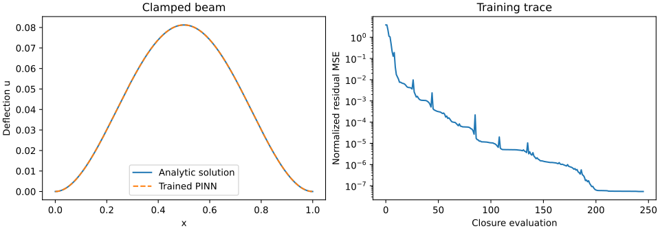
CPU · float64 · one Torch thread · seed recorded in source · 1.64 s for this validation run, excluding imports and figure export. Runtime is a local observation, not a comparative benchmark.
Verified 2026-10-04 against omnibias-torch==0.5.0rc1 and torch==2.14.1+cu130. License: Apache-2.0.
A smooth, nondimensional, manufactured beam problem. Exact boundary conditions come from its polynomial envelope; global PDE convergence is not implied.
The equation and boundary conditions
Use a nondimensional Euler–Bernoulli model with constant flexural rigidity EI = 1:
u''''(x) = q(x),      0 ≤ x ≤ 1
u(0) = u'(0) = u(1) = u'(1) = 0
u*(x) = x²(1 − x)² [1 + 0.3 sin(πx)]
The code derives q analytically from this manufactured solution. Its nonuniform load makes the problem reproducible without importing experimental data or obscuring the reference error.
Parameterize u = p gθ, where p = x²(1−x)² and gθ is a tanh MLP. The double zeros in p enforce deflection and slope at both endpoints for every set of network parameters. These boundary guarantees come from the parameterization.
Why the derivative representation matters
mlp_jet carries the network’s Taylor coefficients along a direction. In this one-dimensional problem the direction is one. jet_to_tower converts the coefficients into ordinary derivatives; omitting that conversion would produce the wrong fourth derivative by a factorial factor.
The product rule gives:
u'''' = p g'''' + 4 p' g''' + 6 p'' g'' + 4 p''' g' + p'''' g
The resulting expressions retain gradients into weights and biases. L-BFGS uses those gradients to reduce the normalized interior residual. A small probe compares the same fourth derivative with nested Torch autograd before training begins.
Install and run
python -m pip install --pre "omnibias-torch==0.5.0rc1" matplotlib
The tested environment is shown above. For the same plotting environment, also use the recorded notebook requirements.
# %% [markdown]
# # A fourth-order beam PINN, from equation to solution
# Solve u''''(x) = q(x) on [0, 1], with u = u' = 0 at both ends.
# This is a nondimensional clamped Euler–Bernoulli beam with EI = 1.
# We manufacture a nonuniform load from u*(x) = x²(1−x)²[1 + 0.3 sin(πx)].
# Install: python -m pip install --pre "omnibias-torch==0.5.0rc1" matplotlib
# The example uses CPU float64. It demonstrates one smooth problem, not general PDE convergence.
# %%
import json
import os
import time
from importlib.metadata import version
from pathlib import Path
import matplotlib.pyplot as plt
import torch
from omnibias.torch.jet import mlp_jet, jet_to_tower

torch.set_num_threads(1)
torch.manual_seed(42)
dtype = torch.float64
started = time.perf_counter()
weights = [torch.nn.Parameter(torch.randn(16, 1, dtype=dtype)),
           torch.nn.Parameter(torch.randn(16, 16, dtype=dtype) / 4),
           torch.nn.Parameter(torch.randn(1, 16, dtype=dtype) / 4)]
biases = [torch.nn.Parameter(torch.zeros(n, dtype=dtype)) for n in (16, 16, 1)]
parameters = [*weights, *biases]
layers = [(weights[0], biases[0], "tanh"), (weights[1], biases[1], "tanh"),
          (weights[2], biases[2], None)]

def network(x):
    return torch.tanh(torch.tanh(x @ weights[0].T + biases[0]) @ weights[1].T + biases[1]) @ weights[2].T + biases[2]

def envelope(x):
    return [x.square() * (1-x).square(), 2*x-6*x.square()+4*x**3,
            2-12*x+12*x.square(), -12+24*x, torch.full_like(x, 24)]

def exact(x):
    return envelope(x)[0] * (1 + .3 * torch.sin(torch.pi*x))

def load(x):
    p = envelope(x)
    g = [1+.3*torch.sin(torch.pi*x), .3*torch.pi*torch.cos(torch.pi*x),
         -.3*torch.pi**2*torch.sin(torch.pi*x), -.3*torch.pi**3*torch.cos(torch.pi*x),
         .3*torch.pi**4*torch.sin(torch.pi*x)]
    return sum(c*p[k]*g[4-k] for k,c in enumerate([1,4,6,4,1]))

def derivatives(x):
    g = jet_to_tower(mlp_jet(x, torch.ones_like(x), layers, order=4))
    assert g.shape == (5, len(x), 1)
    p = envelope(x)
    u = p[0]*g[0]
    fourth = sum(c*p[k]*g[4-k] for k,c in enumerate([1,4,6,4,1]))
    return u, fourth

# %% [markdown]
# ## Independently check the operator, then train
# The polynomial envelope enforces all four boundary conditions for every parameter value.
# omnibias supplies derivatives of the neural factor; the product rule supplies u''''.
# Taylor coefficients must be converted with jet_to_tower before using ordinary derivatives.
# %%
probe = torch.linspace(.11, .89, 5, dtype=dtype).reshape(-1,1).requires_grad_()
reference = envelope(probe)[0]*network(probe)
for _ in range(4):
    reference = torch.autograd.grad(reference.sum(), probe, create_graph=True)[0]
torch.testing.assert_close(derivatives(probe)[1], reference, rtol=1e-8, atol=1e-9)
x_train = torch.linspace(.01, .99, 80, dtype=dtype).reshape(-1,1)
forcing = load(x_train)
optimizer = torch.optim.LBFGS(parameters, lr=1, max_iter=300, tolerance_grad=1e-10,
                             tolerance_change=1e-13, line_search_fn="strong_wolfe")
history = []
def closure():
    optimizer.zero_grad()
    residual = (derivatives(x_train)[1] - forcing) / 24
    loss = residual.square().mean()
    loss.backward()
    assert all(p.grad is not None and torch.isfinite(p.grad).all() for p in parameters)
    history.append(float(loss.detach()))
    return loss
closure()
optimizer.step(closure)

# %% [markdown]
# ## Evaluate unseen coordinates and the physical constraints
# Require relative L2 error below 1%, normalized residual RMS below 1%, and exact boundary values.
# These are sampled checks against a known solution, not a certified global error bound.
# %%
x = torch.linspace(0, 1, 241, dtype=dtype).reshape(-1,1)
prediction, fourth = derivatives(x)
truth = exact(x)
relative_l2 = float((prediction-truth).norm().detach()/truth.norm())
residual_rms = float(((fourth-load(x))/24).square().mean().sqrt().detach())
ends = torch.tensor([[0.], [1.]], dtype=dtype, requires_grad=True)
boundary = envelope(ends)[0]*network(ends)
slopes = torch.autograd.grad(boundary.sum(), ends)[0]
assert relative_l2 < .01, relative_l2
assert residual_rms < .01, residual_rms
torch.testing.assert_close(boundary, torch.zeros_like(boundary), atol=1e-14, rtol=0)
torch.testing.assert_close(slopes, torch.zeros_like(slopes), atol=1e-14, rtol=0)
seconds = time.perf_counter()-started
out = Path(os.environ.get("OMNIBIAS_EXAMPLE_OUTPUT", "omnibias-results")); out.mkdir(parents=True, exist_ok=True)
data = {"id":"beam-pinn", "seed":42, "dtype":"float64", "device":"CPU", "threads":1,
        "packages":{"torch":torch.__version__, "omnibias-torch":version("omnibias-torch")},
        "seconds":seconds, "closure_evaluations":len(history),
        "metrics":{"relative_l2":relative_l2,"normalized_residual_rms":residual_rms,"boundary_max":float(boundary.abs().max().detach())},
        "x":x.flatten().tolist(), "reference":truth.flatten().tolist(), "prediction":prediction.detach().flatten().tolist(), "loss":history}
(out/"beam-pinn.json").write_text(json.dumps(data, indent=2)+"\n")
fig, axes = plt.subplots(1,2,figsize=(10,3.5),layout="constrained")
axes[0].plot(data["x"],data["reference"],label="Analytic solution"); axes[0].plot(data["x"],data["prediction"],"--",label="Trained PINN")
axes[0].set(xlabel="x",ylabel="Deflection u",title="Clamped beam"); axes[0].legend()
axes[1].semilogy(history); axes[1].set(xlabel="Closure evaluation",ylabel="Normalized residual MSE",title="Training trace")
fig.savefig(out/"beam-pinn.svg"); plt.close(fig)
print(json.dumps({"metrics":data["metrics"],"seconds":seconds},indent=2))

# Display the saved scientific figure when running as a Jupyter notebook.
if "get_ipython" in globals():
    from IPython.display import SVG, display
display(SVG(filename=str(out/"beam-pinn.svg")))The notebook and this displayed source are generated from the same executable file. Source SHA-256: 6786d96c1d452e8a96728b69e0116f70f2e10bab3562902185951d1e9a2d6c41.
python beam_pinn.pyFigures and JSON results are written to omnibias-results/. Override that directory with OMNIBIAS_EXAMPLE_OUTPUT. The notebook displays the saved figure after execution.
What the assertions establish
The derivative tower has shape (5, batch, 1). Its fourth derivative agrees with an independent autograd calculation within float64 tolerances. Every parameter receives finite gradients. Validation uses 241 coordinates and requires relative solution error below 1% and normalized residual RMS below 1%. Endpoint deflection and slope must be zero to absolute tolerance 1e-14.
Sampled error is distinct from a certified global bound. Changing the load, activation, geometry, stiffness, or conditioning requires a new validation problem. This small smooth beam also does not measure general training-speed gains.
When should I use this PINN example?
Use it as a reproducible starting point for a one-dimensional fourth-order residual with trainable network parameters. The exact boundary envelope applies to the clamped endpoints shown here. A different support condition, variable stiffness, or physical scale changes the residual or parameterization and needs fresh validation against an independent solution.
Related APIs and examples
PyTorch jet API · Trainable residual foundations · Poisson with a direct Laplacian · Scientific ML notebooks