Calibrate a scientific model with Gauss–Newton
Scientific calibration turns observations into model parameters. This small nonlinear least-squares problem recovers an amplitude, decay rate, and offset, with independently checked sensitivities and a known answer.
Recover amplitude, decay rate, and offset in a nonlinear least-squares inverse problem using a verified residual Jacobian and functional Gauss–Newton steps.
CPU · float64 · one Torch thread · seed recorded in source · 0.88 s for this validation run, excluding imports and figure export. Runtime is a local observation, not a comparative benchmark.
Verified 2026-10-04 against omnibias-torch==0.5.0rc1 and torch==2.14.1+cu130. License: Apache-2.0.
Three parameters and noiseless synthetic decay observations. Recovery at floating-point precision is not a robustness or uncertainty guarantee for noisy measurements.
Formulate the inverse problem
y(t) = A exp(−kt) + b
residual_i(θ) = model(θ, t_i) − observed_i
A = exp(θ₀), k = exp(θ₁), b = θ₂
The observations are noiseless synthetic samples with A = 2, k = 0.7, and b = 0.2. Positive amplitude and rate are enforced by the log parameterization. The offset remains unconstrained.
Before optimization, the code compares torch.func.jacrev(residual) with the explicit analytic residual Jacobian. This catches errors in parameterization and chain-rule factors. A separate check confirms finite, nonzero parameter gradients at initialization.
Use the functional optimizer contract
GaussNewton(solver="qr", damping=1e-3) acts on a residual closure and a flat parameter vector. Each step returns a new parameter vector and diagnostic information. It does not mutate the weights of an nn.Module for you.
The method uses residual-Jacobian curvature. The full Hessian of a nonlinear least-squares loss has an additional residual-weighted second-derivative term; the two are not generally identical.
Install and run
python -m pip install --pre "omnibias-torch==0.5.0rc1" matplotlib
# %% [markdown]
# # Calibrate a decay model with Gauss–Newton
# Recover amplitude A, rate k, and offset b from y(t) = A exp(−kt) + b.
# These noiseless synthetic observations provide a checkable inverse problem.
# Install: python -m pip install --pre "omnibias-torch==0.5.0rc1" matplotlib
# Gauss–Newton uses residual-Jacobian curvature. It is distinct from the full loss Hessian.
# %%
import json
import os
import time
from pathlib import Path
from importlib.metadata import version
import matplotlib.pyplot as plt
import torch
from omnibias.torch.optim import GaussNewton

torch.set_num_threads(1); torch.manual_seed(31)
dtype = torch.float64
started = time.perf_counter()
t = torch.linspace(0,5,60,dtype=dtype)
truth = torch.tensor([2.,.7,.2],dtype=dtype)
observed = truth[0]*torch.exp(-truth[1]*t)+truth[2]
def physical(theta):
    return torch.stack([theta[0].exp(),theta[1].exp(),theta[2]])
def model(theta,time):
    a,k,b = physical(theta).unbind()
    return a*torch.exp(-k*time)+b
def residual(theta):
    return model(theta,t)-observed
theta = torch.tensor([1.2,.5,.1],dtype=dtype)
theta[:2] = theta[:2].log()
initial = model(theta,t).detach()

# %% [markdown]
# ## Check parameter sensitivities and take functional steps
# step returns a new flat vector; it does not mutate an nn.Module.
# Log parameterization keeps amplitude and decay rate positive. The offset is unconstrained.
# %%
jacobian = torch.func.jacrev(residual)(theta)
a,k,b = physical(theta).unbind()
expected = torch.stack([a*torch.exp(-k*t),-a*k*t*torch.exp(-k*t),torch.ones_like(t)],1)
torch.testing.assert_close(jacobian,expected,rtol=1e-10,atol=1e-12)
probe = theta.clone().requires_grad_()
gradient = torch.autograd.grad(residual(probe).square().mean(),probe)[0]
assert torch.isfinite(gradient).all() and bool((gradient.abs()>0).all())
optimizer = GaussNewton(solver="qr",damping=1e-3)
history = [float(residual(theta).square().mean())]
for _ in range(12):
    theta,info = optimizer.step(residual,theta)
    history.append(float(residual(theta).square().mean().detach()))
recovered = physical(theta).detach()
torch.testing.assert_close(recovered,truth,rtol=1e-6,atol=1e-7)
heldout = torch.linspace(.025,4.975,101,dtype=dtype)
heldout_rmse = float((model(theta,heldout)-(truth[0]*torch.exp(-truth[1]*heldout)+truth[2])).square().mean().sqrt().detach())
assert heldout_rmse < 1e-6
assert history[-1] < history[0]
seconds = time.perf_counter()-started
out = Path(os.environ.get("OMNIBIAS_EXAMPLE_OUTPUT","omnibias-results")); out.mkdir(parents=True,exist_ok=True)
data = {"id":"decay-calibration","seed":31,"dtype":"float64","device":"CPU","threads":1,
        "packages":{"torch":torch.__version__,"omnibias-torch":version("omnibias-torch")},
        "seconds":seconds,"steps":12,"metrics":{"heldout_rmse":heldout_rmse,"max_parameter_error":float((recovered-truth).abs().max())},
        "recovered_parameters":recovered.tolist(),"x":t.tolist(),"reference":observed.tolist(),"initial":initial.tolist(),"prediction":model(theta,t).detach().tolist(),"loss":history}
(out/"decay-calibration.json").write_text(json.dumps(data,indent=2)+"\n")
fig,axes = plt.subplots(1,2,figsize=(10,3.5),layout="constrained")
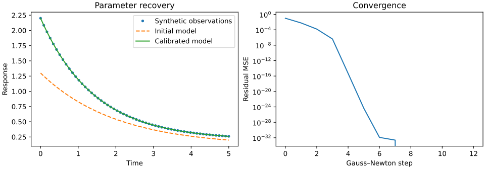
axes[0].plot(data["x"],data["reference"],".",label="Synthetic observations"); axes[0].plot(data["x"],data["initial"],"--",label="Initial model"); axes[0].plot(data["x"],data["prediction"],label="Calibrated model"); axes[0].legend(); axes[0].set(xlabel="Time",ylabel="Response",title="Parameter recovery")
axes[1].semilogy(history); axes[1].set(xlabel="Gauss–Newton step",ylabel="Residual MSE",title="Convergence")
fig.savefig(out/"decay-calibration.svg"); plt.close(fig)
print(json.dumps({"metrics":data["metrics"],"seconds":seconds,"recovered":recovered.tolist()},indent=2))

# Display the saved scientific figure when running as a Jupyter notebook.
if "get_ipython" in globals():
    from IPython.display import SVG, display
display(SVG(filename=str(out/"decay-calibration.svg")))The notebook and this displayed source are generated from the same executable file. Source SHA-256: 99ae3ad446cf093b0f0e17f12385f048f37034b3a4a40624ce61f3c4468aa4bd.
python decay_calibration.pyFigures and JSON results are written to omnibias-results/. Override that directory with OMNIBIAS_EXAMPLE_OUTPUT. The notebook displays the saved figure after execution.
What successful recovery means
After 12 steps, parameter values must agree with the known target within rtol=1e-6 and atol=1e-7. Predictions on 101 additional times must have RMSE below 1e-6. The recorded run recovers the displayed parameters to floating-point precision.
Real calibration work must also consider observation noise, identifiability, parameter correlations, outliers, initialization, and model mismatch. Exact recovery on noiseless synthetic data does not supply uncertainty estimates or guarantee recovery on experimental observations.
How does this relate to differential-equation parameter estimation?
Exponential decay solves the first-order equation dy/dt = -k(y-b). This example calibrates its analytic solution directly rather than differentiating through an ODE solver. For a model without an analytic solution, the residual closure must include a suitable solver or surrogate and valid parameter sensitivities. The synthetic recovery test here is a checkable starting point for that larger inverse problem.
Related APIs and examples
Optimization API · Second-order optimization contracts · Scientific ML notebooks