A Poisson PINN without a full Hessian
When a residual needs a Laplacian, the relevant quantity is the sum of the diagonal spatial second derivatives. A supported direct contraction can compute that quantity without constructing every Hessian entry in the training loop.
Train a two-dimensional Poisson PINN using direct Laplacian contraction, then inspect solution error, boundary error, and residual error separately.
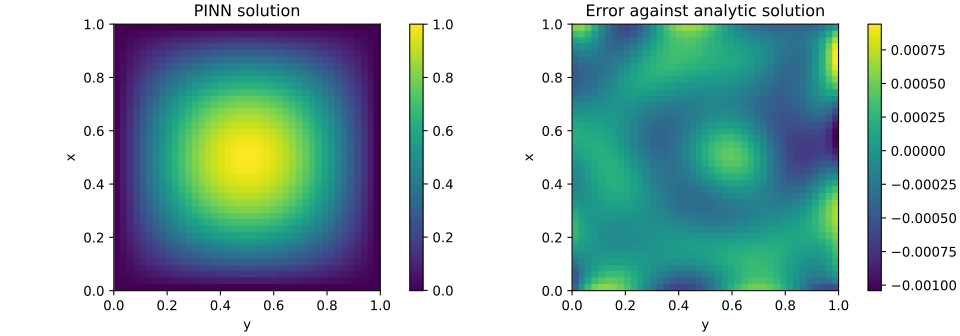
CPU · float64 · one Torch thread · seed recorded in source · 2.41 s for this validation run, excluding imports and figure export. Runtime is a local observation, not a comparative benchmark.
Verified 2026-10-04 against omnibias-torch==0.5.0rc1 and torch==2.14.1+cu130. License: Apache-2.0.
A unit-square Poisson problem with a known smooth solution. Boundary values are penalized, not exactly enforced. This is not a measured training-speed comparison.
Define a checkable field equation
Δu(x,y) = −2π² sin(πx) sin(πy),    (x,y) ∈ [0,1]²
u = 0 on the boundary
u*(x,y) = sin(πx) sin(πy)
Poisson equations appear in potential fields and steady diffusion formulations. This tutorial uses a manufactured solution to make numerical error visible; it is not a validated model of a particular physical device.
The network has two input coordinates, two 24-unit tanh hidden layers, and one output. Layer weights use (out_features, in_features). deep_field_laplacian(points, layers) returns (batch, 1) for this architecture.
Keep boundary and interior objectives separate
The interior loss is the mean squared PDE residual divided by (2π²)². A weighted boundary penalty adds 5 * mean(u_boundary²). That weight is a modelling choice, not an exact boundary guarantee.
Before training, three probes compare the direct Laplacian against the trace of a dense Hessian computed independently with torch.func.hessian. Dense Hessians are used only for that small check. L-BFGS then trains the direct-contraction residual, with assertions that every parameter receives finite gradients.
Install and run
python -m pip install --pre "omnibias-torch==0.5.0rc1" matplotlib
# %% [markdown]
# # A Poisson PINN with a direct Laplacian
# Solve Δu = −2π² sin(πx)sin(πy) on the unit square, with u = 0 on the boundary.
# The known solution sin(πx)sin(πy) lets us evaluate unseen coordinates independently.
# Install: python -m pip install --pre "omnibias-torch==0.5.0rc1" matplotlib
# CPU float64. Direct contraction avoids forming a full Hessian in the training residual.
# %%
import json
import os
import time
from pathlib import Path
from importlib.metadata import version
import matplotlib.pyplot as plt
import torch
from omnibias.torch.laplacian import deep_field_laplacian

torch.set_num_threads(1)
torch.manual_seed(17)
dtype = torch.float64
started = time.perf_counter()
weights = [torch.nn.Parameter(torch.randn(24,2,dtype=dtype)),
           torch.nn.Parameter(torch.randn(24,24,dtype=dtype)/5),
           torch.nn.Parameter(torch.randn(1,24,dtype=dtype)/5)]
biases = [torch.nn.Parameter(torch.zeros(n,dtype=dtype)) for n in (24,24,1)]
parameters = [*weights,*biases]
layers = [(weights[0],biases[0],"tanh"),(weights[1],biases[1],"tanh"),(weights[2],biases[2],None)]
def model(x):
    return torch.tanh(torch.tanh(x@weights[0].T+biases[0])@weights[1].T+biases[1])@weights[2].T+biases[2]
def exact(x):
    return torch.sin(torch.pi*x[:,0:1])*torch.sin(torch.pi*x[:,1:2])
def grid(axis):
    return torch.stack(torch.meshgrid(axis,axis,indexing="ij"),-1).reshape(-1,2)

# %% [markdown]
# ## Check the contraction against an independent Hessian
# Only three probe points use a dense Hessian. The residual uses deep_field_laplacian.
# This test validates the operator for this architecture and dtype, not every possible model.
# %%
probe = torch.tensor([[.17,.29],[.53,.71],[.83,.37]],dtype=dtype)
dense = torch.stack([torch.func.hessian(lambda z:model(z[None]).squeeze())(p).trace() for p in probe])
torch.testing.assert_close(deep_field_laplacian(probe,layers).flatten(),dense,rtol=1e-9,atol=1e-10)
interior = grid(torch.linspace(.025,.975,15,dtype=dtype))
edge = torch.linspace(0,1,25,dtype=dtype)
boundary = torch.cat([torch.stack([edge,torch.zeros_like(edge)],1),torch.stack([edge,torch.ones_like(edge)],1),
                      torch.stack([torch.zeros_like(edge),edge],1),torch.stack([torch.ones_like(edge),edge],1)])
forcing = -2*torch.pi**2*exact(interior)
optimizer = torch.optim.LBFGS(parameters,lr=1,max_iter=600,tolerance_grad=1e-10,
                             tolerance_change=1e-13,line_search_fn="strong_wolfe")
history = []
def closure():
    optimizer.zero_grad()
    residual = (deep_field_laplacian(interior,layers)-forcing)/(2*torch.pi**2)
    loss = residual.square().mean()+5*model(boundary).square().mean()
    loss.backward()
    assert all(p.grad is not None and torch.isfinite(p.grad).all() for p in parameters)
    history.append(float(loss.detach()))
    return loss
closure(); optimizer.step(closure)

# %% [markdown]
# ## Validate interior error and boundary error separately
# Boundary conditions are penalized, not structurally exact. We report their maximum error.
# No end-to-end speedup is claimed: this notebook establishes a complete, trainable workflow.
# %%
axis = torch.linspace(0,1,41,dtype=dtype)
points = grid(axis)
prediction = model(points).detach(); truth = exact(points)
relative_l2 = float((prediction-truth).norm()/truth.norm())
boundary_max = float(model(boundary).detach().abs().max())
residual_rms = float(((deep_field_laplacian(points,layers).detach()+2*torch.pi**2*truth)/(2*torch.pi**2)).square().mean().sqrt())
assert relative_l2 < .02, relative_l2
assert boundary_max < .02, boundary_max
assert residual_rms < .03, residual_rms
seconds = time.perf_counter()-started
out = Path(os.environ.get("OMNIBIAS_EXAMPLE_OUTPUT","omnibias-results")); out.mkdir(parents=True,exist_ok=True)
data = {"id":"poisson-pinn","seed":17,"dtype":"float64","device":"CPU","threads":1,
        "packages":{"torch":torch.__version__,"omnibias-torch":version("omnibias-torch")},
        "seconds":seconds,"closure_evaluations":len(history),
        "metrics":{"relative_l2":relative_l2,"boundary_max":boundary_max,"normalized_residual_rms":residual_rms},
        "axis":axis.tolist(),"prediction":prediction.reshape(41,41).tolist(),"error":(prediction-truth).reshape(41,41).tolist(),"loss":history}
(out/"poisson-pinn.json").write_text(json.dumps(data,indent=2)+"\n")
fig,axes = plt.subplots(1,2,figsize=(10,3.5),layout="constrained")
for ax,values,title in [(axes[0],data["prediction"],"PINN solution"),(axes[1],data["error"],"Error against analytic solution")]:
    im=ax.imshow(values,origin="lower",extent=[0,1,0,1]); ax.set(xlabel="y",ylabel="x",title=title); fig.colorbar(im,ax=ax)
fig.savefig(out/"poisson-pinn.svg"); plt.close(fig)
print(json.dumps({"metrics":data["metrics"],"seconds":seconds},indent=2))

# Display the saved scientific figure when running as a Jupyter notebook.
if "get_ipython" in globals():
    from IPython.display import SVG, display
display(SVG(filename=str(out/"poisson-pinn.svg")))The notebook and this displayed source are generated from the same executable file. Source SHA-256: d829fe50a10a8013e8734711c44dd2b73097ea432ad5692d3e83a5092a66e83c.
python poisson_pinn.pyFigures and JSON results are written to omnibias-results/. Override that directory with OMNIBIAS_EXAMPLE_OUTPUT. The notebook displays the saved figure after execution.
Read the result correctly
The final 41 × 41 grid measures relative solution error and normalized residual RMS. The boundary maximum is reported separately. The assertions require relative solution error below 2%, boundary error below 0.02, and normalized residual RMS below 0.03.
The current recorded run is substantially below those limits. Reproduce it before changing collocation points, dtype, architecture, or penalty weights. This notebook establishes a complete workflow; it does not compare training speed against another solver. Direct contractions still have costs that depend on dimension, width, depth, and the supported representation.
Does avoiding a Hessian change the PDE?
The direct operator computes the same supported Laplacian quantity; the small independent trace check verifies that equivalence for this architecture. The PDE, boundary penalty, collocation points, and optimizer remain modeling choices. Compare solution error and runtime on your own equation before concluding that a different derivative representation improves training.
Related APIs and examples
Laplacian API · First Laplacian tutorial · Measured operator benchmarks · Scientific ML notebooks