Train differentiable regions and local experts
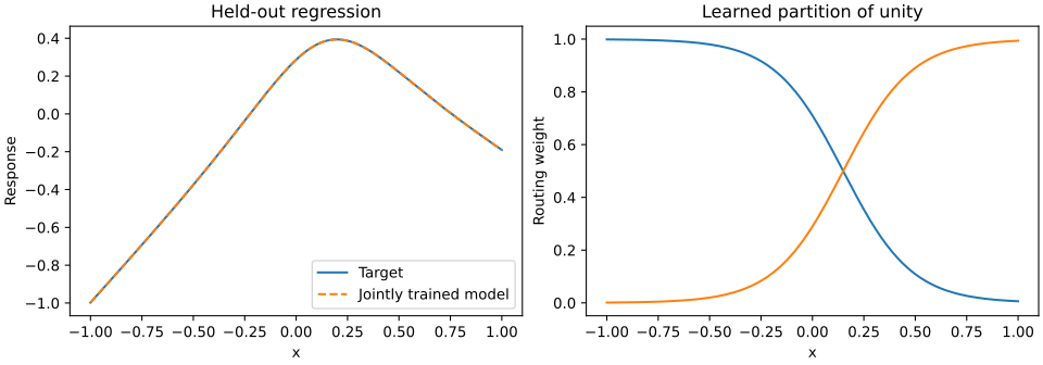
A regional model can learn both its local responses and where those responses apply. This example trains a smooth split, threshold, and two linear experts together, then checks predictions on a separate grid.
Learn a soft split and two regional regressors together, validate held-out predictions, and measure what changes when routing is hardened.
CPU · float64 · one Torch thread · seed recorded in source · 1.77 s for this validation run, excluding imports and figure export. Runtime is a local observation, not a comparative benchmark.
Verified 2026-10-04 against omnibias-torch==0.5.0rc1 and torch==2.14.1+cu130. License: AGPL-3.0-or-later / commercial.
Synthetic two-regime regression, not an industrial deployment. Increasing the inverse temperature changes the model and can increase prediction error.
The target and model
The manufactured target blends two linear responses around x = 0.15, using inverse temperature β = 6. The training inputs are 160 seeded samples from [-1,1]. A separate 301-point grid evaluates generalization within that interval.
partition_weights_arrays produces a (batch, 2) array for a depth-one split. Its nonnegative rows sum to one. combine blends the expert outputs into a (batch,) prediction. The trainable quantities are the split direction W, threshold, expert slopes, and expert offsets.
This is a minimal example of regime-dependent behaviour, relevant to thinking about piecewise responses and local surrogate models. It uses synthetic data and provides no evidence of performance on a particular industrial dataset.
Install and review the license
python -m pip install --pre "omnibias-torch==0.5.0rc1" "omnibias-partition==0.1.0a2" matplotlib
The partition extension is an alpha distribution under AGPL-3.0-or-later or a commercial license. Its license differs from the Apache-2.0 Torch substrate. Read the licensing overview before choosing it for your application.
# %% [markdown]
# # Learn a split and its regional experts together
# A manufactured two-regime regression problem illustrates smooth, trainable routing.
# The target blends two linear responses around x = 0.15. It is not an industrial case study.
# Install: python -m pip install --pre "omnibias-torch==0.5.0rc1" "omnibias-partition==0.1.0a2" matplotlib
# The partition package is AGPL-3.0-or-later or commercially licensed; review its license for your application.
# %%
import json
import os
import time
from pathlib import Path
from importlib.metadata import version
import matplotlib.pyplot as plt
import torch
from omnibias.partition.torch.weights import partition_weights_arrays, combine

torch.set_num_threads(1); torch.manual_seed(23)
dtype = torch.float64
started = time.perf_counter()
W = torch.nn.Parameter(torch.tensor([[.65]],dtype=dtype))
threshold = torch.nn.Parameter(torch.tensor([-.2],dtype=dtype))
slopes = torch.nn.Parameter(torch.tensor([.2,-.1],dtype=dtype))
offsets = torch.nn.Parameter(torch.zeros(2,dtype=dtype))
parameters = [W,threshold,slopes,offsets]
def target(x):
    weights = partition_weights_arrays(torch.ones(1,1,dtype=dtype),torch.tensor([.15],dtype=dtype),x,beta=6.,depth=1)
    return combine(weights,x*torch.tensor([1.2,-.7],dtype=dtype)+torch.tensor([.2,.5],dtype=dtype))
def predict(x,beta=6.):
    weights = partition_weights_arrays(W,threshold,x,beta=beta,depth=1)
    return combine(weights,x*slopes+offsets),weights

# %% [markdown]
# ## Train on sampled points, evaluate on a separate grid
# Gradients reach split direction, threshold, slopes, and offsets. Nonnegative routing weights sum to one.
# Raising beta later sharpens routing but changes the represented function; it is not a free accuracy improvement.
# %%
train = 2*torch.rand(160,1,dtype=dtype)-1
labels = target(train)
optimizer = torch.optim.Adam(parameters,lr=.025)
history = []
for step in range(1800):
    optimizer.zero_grad()
    prediction,weights = predict(train)
    loss = (prediction-labels).square().mean()
    loss.backward()
    assert all(p.grad is not None and torch.isfinite(p.grad).all() for p in parameters)
    optimizer.step()
    if step % 10 == 0: history.append(float(loss.detach()))
x = torch.linspace(-1,1,301,dtype=dtype).reshape(-1,1)
prediction,weights = predict(x); truth = target(x)
torch.testing.assert_close(weights.sum(-1),torch.ones(len(x),dtype=dtype),rtol=1e-12,atol=1e-12)
assert bool((weights>=0).all())
rmse = float((prediction-truth).square().mean().sqrt().detach())
assert rmse < .015, rmse
sharp,_ = predict(x,beta=24.)
sharp_rmse = float((sharp-truth).square().mean().sqrt().detach())
seconds = time.perf_counter()-started
out = Path(os.environ.get("OMNIBIAS_EXAMPLE_OUTPUT","omnibias-results")); out.mkdir(parents=True,exist_ok=True)
data = {"id":"regional-regression","seed":23,"dtype":"float64","device":"CPU","threads":1,
        "packages":{"torch":torch.__version__,"omnibias-torch":version("omnibias-torch"),"omnibias-partition":version("omnibias-partition")},
        "seconds":seconds,"steps":1800,"metrics":{"heldout_rmse":rmse,"hardened_rmse":sharp_rmse},
        "x":x.flatten().tolist(),"reference":truth.tolist(),"prediction":prediction.detach().tolist(),
        "weights":weights.detach().tolist(),"hardened":sharp.detach().tolist(),"loss":history}
(out/"regional-regression.json").write_text(json.dumps(data,indent=2)+"\n")
fig,axes = plt.subplots(1,2,figsize=(10,3.5),layout="constrained")
axes[0].plot(data["x"],data["reference"],label="Target"); axes[0].plot(data["x"],data["prediction"],"--",label="Jointly trained model"); axes[0].legend(); axes[0].set(xlabel="x",ylabel="Response",title="Held-out regression")
axes[1].plot(data["x"],data["weights"]); axes[1].set(xlabel="x",ylabel="Routing weight",title="Learned partition of unity")
fig.savefig(out/"regional-regression.svg"); plt.close(fig)
print(json.dumps({"metrics":data["metrics"],"seconds":seconds},indent=2))

# Display the saved scientific figure when running as a Jupyter notebook.
if "get_ipython" in globals():
    from IPython.display import SVG, display
display(SVG(filename=str(out/"regional-regression.svg")))The notebook and this displayed source are generated from the same executable file. Source SHA-256: 2208b2473618dc65a1abce7d774c09a4bc217cf009cb62661e0d58ee5170e3da.
python regional_regression.pyFigures and JSON results are written to omnibias-results/. Override that directory with OMNIBIAS_EXAMPLE_OUTPUT. The notebook displays the saved figure after execution.
Soft training and hardening are different experiments
The training loop checks finite gradients into all four parameter groups and requires held-out RMSE below 0.015. It also checks nonnegative weights and their partition-of-unity identity.
The final model is evaluated again with inverse temperature 24. The sharper routing has a different output and a separately recorded error. In the recorded run it increases error, demonstrating why a hardening schedule must be validated against the actual objective.
Temperature hardening sharpens an existing smooth model. It does not differentiate a pre-existing hard discontinuity. Bias collapse, the separate mathematical limit used to extract derivatives, should not be confused with this operation.
Continue
Partition weights API · Soft regional model foundations · Hard quantization contracts · Scientific ML notebooks